Predicting water solubility - Part II?
Feature selection


- Requirements
- Background
- Import modules
- Load Data
- Featurization
- Understanding the features
- In depth analysis of feature correlation
- Training a baseline model
- Feature selection
- Final selection of features
- What method should I use?
- Conclusion
- References
- Fin
- rdkit >= 2020.09.1
- pandas >= 1.1.3
- seaborn
- matplotlib
- fastcore (!conda install fastcore)
In this tutorial we'll use a dataset compiled by Sorkun et al (2019) from multiple projects to predict water solubility. You can download the original dataset from here.
At the end of the notebook I added a class to process the original dataset in order to remove salts, mixtures, neutralize charges and generate canonical SMILES. I highly recommend checking each structure before modeling.
In this notebook we'll cover three main topics:
- Featurization of molecules
- What's the correlation between features?
- Feature selection methods
Drug solubility is a critical factor in drug development. If a drug is not soluble enough or doesn't dissolve readily its intestinal absoption will be compromised, leading to low concentration in the blood circulation and reduced (or none) biological activity.
Crystal formation of low soluble drugs may also lead to toxicity. In practical terms, poor solubility is one of the factors that lead to fail in drug discovery projects. Therefore, medicinal chemists work hard to design molecules tha have the intended bioactivity and that can display the desired effect in vivo.
Despite being conceptually easy to understand solubility, its estimation isn't easy. That's because the intrinsic solubility of a molecule depends on many factors, including its size, shape, the ability to make intermolecular interactions and crystal packing.
%reload_ext autoreload
%autoreload 2
%matplotlib inline
from IPython.display import Image
import matplotlib.pyplot as plt
from matplotlib.ticker import FormatStrFormatter
import seaborn as sns
import pandas as pd
import numpy as np

from sklearn.preprocessing import Normalizer, normalize, RobustScaler
from sklearn.ensemble import RandomForestRegressor
from xgboost import XGBRegressor
from sklearn.metrics import make_scorer, mean_squared_error

from sklearn.feature_selection import mutual_info_regression, RFECV,SelectFromModel,RFE,VarianceThreshold
from functools import partial
from pathlib import Path
from joblib import load, dump

from scipy import stats
from scipy.stats import norm
from statsmodels.graphics.gofplots import qqplot
from rdkit.Chem import Draw
from rdkit.Chem import MolFromSmiles, MolToSmiles

from descriptastorus.descriptors.DescriptorGenerator import MakeGenerator
np.random.seed(5)
sns.set(rc={'figure.figsize': (16, 16)})
sns.set_style('whitegrid')
sns.set_context('paper',font_scale=1.5)
Let's load the dataset without outliers from the last post.
data = pd.read_csv('../_data/water_solubility_nooutliers.csv')
data.head()
In this dataset 17 features were already calculated for each molecule. These features include a range of physichochemical properties (e.g. MolWt, MolLogP and MolMR), atomic counts (e.g. HeavyAtomCount, NumHDonors and Acceptors) and more abstract topological descriptors (e.g. BalabanJ, BertzCT).
descriptors = ['MolWt', 'MolLogP', 'MolMR', 'HeavyAtomCount',
       'NumHAcceptors', 'NumHDonors', 'NumHeteroatoms', 'NumRotatableBonds',
       'NumValenceElectrons', 'NumAromaticRings', 'NumSaturatedRings',
       'NumAliphaticRings', 'RingCount', 'TPSA', 'LabuteASA', 'BalabanJ',
       'BertzCT']

var =  ['Solubility']+ descriptors
print(len(descriptors))
We can check the correlation between each feature and solubility using seaborn's regplot:
nr_rows = 6
nr_cols = 3
target = 'Solubility'

Most features have a negative correlation with solubility. In fact, the available features reflect more or less the size/complexity of the molecule (e.g. MolWt, RingCount, MolMR) and it's capacity to make inter and intramolecular interactions (e.g., NumValenceElectrons, NumHAcceptors, NumHDonors, MolLogP), which are known to influence water solubility. For instance, bigger molecules tend to be less soluble in water (high MolMW and HeavyAtomCount); the same applies for very liphophilic (high MolLogP) molecules. On the other hand, more polar molecules, capable of making hydrogen bonds with water, are usually more soluble.
Based on this preliminary analysis we can start thinking which features to include when training a regression model. For instance, molecular weight and liphophilicity are the features most correlated with the target variable. These features have a strong influence in solubility as demonstrated experimentally and by theorical calculations. As the molecular size and liphophilicity grows, its much harder to dissolve a molecule in water because the solute needs to disrupt a great number interactions within solvent molecules and force its way into bulk water, which demands a great amount of energy. The influence of lipophilicity is so well known that its part of many predictive models, such as the famous ESOL (estimated solubility), which estimates water solubility based only on the molecular structure.
Back in the day (2003!) the author of ESOL didn't even use the robust machine learning algorithms we have today to derive the following equation:
$$logS_{w} = 0.16 - 0.63logP - 0.0062MolWt + 0.066Rot - -0.74AP$$
where $logS_{w}$ is the log of the water solubility, $logP$ is the lipophilicity, $MolWt$ is the molecular weight, $Rot$ is the number of rotatable bonds (e.g. single bonds) and $AP$ is the proportion of heavy atoms that are part of aromatic rings.
1) LogP
The logP is the partition coefficient given by:
$$logP = \frac{C_{n-octanol}}{C_{water}}$$
where $C_{n-octanol}$ and $C_{water}$ are the solute concentration in n-octanol and water, respectively. Thus, higher logP means that a smaller concentration of the molecule is available in the water phase of a system, which makes it more lipophilic or hydrophobic.
2) Molecular weight
Molecular weight (MolWt) is simply the total mass of a mole) of a compound. The MolWt can be calculated by the summing the mass contribution of each atom in a molecule. For example, the molar weight of water is:
$$H_{2}O = 2H * (1.01 g/mol) + 1O * (16 g/mol) = 18.01 g/mol$$
3) Molar refractivity
Molar refractivity (MolMR) is the refractivity of a mole of a substance and is a measure of polarizability. It's given by the formula:
$$MolMR = \frac{n^{2}-1}{n^{2}+2}*\frac{MolWt}{d}$$
where $MolWt$ is the molar weight, $d$ is the density and $n$ is the refractivity index. The right hand side of the equation ($\frac{MolWt}{d}$) is the volume. Thus, the molar refractivity encodes the molecular volume and is a way to estimate the steric bulk.
4) Topological polar surface area (TPSA) and LabuteASA
- TPSA: The polar surface area is the sum of the surfaces of polar atoms in a molecule, such as oxygen and nitrogen, and sometimes sulphur and its hydrogen. The total polar surface area is a useful feature to encode both the polarity and the hydrogen bonding capacity of a molecule.
- LabuteASA: the accessible surface area (ASA) is the area of a molecule that is accessible to the solvent (e.g. water). The ASA is calculated by summing the surface area of each atom in a molecule. We can also think about ASA as the area a water molecule can touch as we roll it on the surface of the solute.
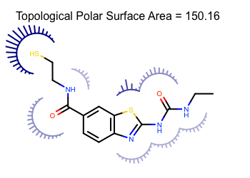
Figure 1. Representation of the polar surface area, showing the contributions of each polar atom in the molecule.
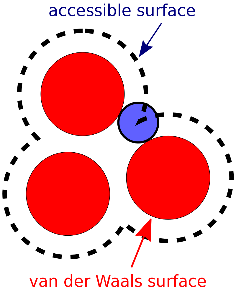
Figure 2. Representation of the polar surface area, showing the contributions of each polar atom in the molecule.
6) Topological descriptors
Topological descriptors in this dataset include BalabanJ and BertzCT and represent more abstract definition of a molecule. For the BalabanJ, the feature value is calculated from the distance matrix, a n x n matrix where n is the number of atoms and the entries represent the distances between each atom in the molecular graph. The BalabanJ descriptor can thus capture topological information such as branching, distance between substructures and the molecular size. The BertzCT descriptor encodes the molecular complexity by taking into account bond connectivity and atom types.
Now let's get to work!
First, let's calculate the Pearson's R coefficient for each pair of features and visualize the results using a heatmap.
The largest diagonal corresponds to self correlation for each feature (e.g. MolWt x MolWt), and is always 1. The most interesting part are the other values, showing the correlation between each pair of features and target variable.
As we can see from the heatmap, some features have a high negative linear correlation with solubility, such as MolWt (-0.61), LabuteASA (-0.62), MolLogP (-0.78) and MolMR (-0.64), HeavyAtomCount (-0.57).
We can also investigate the correlations between features. For the BalabanJ descriptor, the highest correlation was with RingCount (-0.64). For BertzCT, the highest correlations were with features that encode the molecular complexity/size, such as molecular weight, molar refractivity and number of heavy atoms, which is consistent with its definition.
corr = data[var].corr('pearson')
sns.heatmap(corr, annot=True)

We can also see that the number of hydrogen bond donors have a weak positive correlation with solubility, while the number of H-bond acceptors have a very weak negative correlation. This is interesting because it shows us that increasing the H-bond potential might not be the best strategy to increase solubility.
In general, increasing H-bond donors and acceptors also increases solubility because it alters the capacity to make H-bonds with water molecules. However, if the molecule can both donate and accept H-bonds, a decrease in solubility might happen due to intermolecular interactions between molecules of the same kind, leading to reduced ability to be solvated by water molecules. The intuition is that a molecule needs to make better interactions with water than with others of its kind, otherwise it will be poorly solvated.
To summarize this initial analysis, the heatmap give us an idea of what types of features to include in a model. If we were to cherry pick, features like MolLogP, MolMR and LabuteASA would probably be selected. In addition, we must avoid highly correlated features (i.e. that encode the same kind of information) because that would only make our model more complex without any benefit in performance.
But no need to rush! We'll systematically check each feature for better correlations with the target variable and with each other. Remember that our goal is to develop a model with high predictive power, and to do that we need to select the right set of features.
Before we dive into feature selection, let's try a baseline model and see how it performs when training using all features. For this task, we will use the Random Forest algorithm. First, split the data into training and testing sets.
from sklearn.model_selection import train_test_split
trainset, testset = train_test_split(data, test_size = 0.30, random_state=42)
Since our features are in different scales, let's normalize them to have zero mean and unit std. This is an important step so that one feature with large std doesn't dominate the others during training, which could lead to overfitting.
Random forest is robust to the scale of features so this step isn't necessary in this case. We will normalize anyway because it's best practice, especially in models that depends on coefficients and intercepts (e.g. linear regression).
xtrain, xtest = trainset[descriptors].values, testset[descriptors].values
ytrain, ytest = trainset['Solubility'].values, testset['Solubility'].values
We will do the preprocessing in a more compact way by using sklearn pipeline, which will contain the preprocessing steps and a fit call to the training algorithm.
from sklearn.pipeline import Pipeline
pipe = Pipeline(steps=[
    ('scaler',RobustScaler()),
    ('estimator', RandomForestRegressor(n_estimators=2000, n_jobs=-1))
                      ]
               )
We will validate our model using 5-fold cross-validation.
from sklearn.model_selection import cross_val_score
metric = make_scorer(mean_squared_error, squared=False) # RMSE
cross_score = cross_val_score(estimator=pipe, X=xtrain,scoring=metric, y=ytrain, cv=5, n_jobs=-1)
print(f'Mean 5-fold RMSE = {cross_score.mean():.4f}')
Now the test set:
pipe.fit(xtrain,ytrain)
def get_preds(estimator, x):
    preds = estimator.predict(x)
    return preds
preds = pipe.predict(xtest)
print(f'RMSE test set = {mean_squared_error(preds, ytest, squared=False):.3f}')
Not bad! This is our baseline. Let's see if we can beat it or simplify our data a little bit without compromising performance.
yrandom = np.random.choice(ytrain,ytrain.shape[0])
yrandom.shape,ytrain.shape
yrandom, ytrain
pipe.fit(xtrain,yrandom)
preds_random = pipe.predict(xtest)
print(f'RMSE (randomized target) test set = {mean_squared_error(preds_random, ytest, squared=False)}')
As you can see, the RMSE on the test set does increase. In a data set with dozens or even hundreds of features, which is relatively common in QSAR applications, we would expect much higher errors. That's why it's so important to analyze your features carefully in order to remove anything that could hamper performance, including missing or constant values and highly correlated features.
1) Filter methods
Filter methods are the easiest to implement because they are model-agnostic, which means we don't need any fancy learning algorithm. This class of methods consists of statistical approaches that use the distribution of the dataset to remove features that don't have much information or correlation with the target variable. Since we don't need a model, filter methods are very fast and can give an initial guess of what types of features to keep.
Despite being fast, filter methods also come with some dangerous drawbacks. Since most methods are univariate, important correlations between features may be missed; or worse redudant features could be selected. In addition, most metrics (e.g. Pearson's correlation coefficient) used to select the features are subjective and not always correlate with the metric that will be used to access performance.
While filter methods tend to be simple and fast, there is a subjective nature to the procedure. Most scoring methods have no obvious cut point to declare which predictors are important enough to go into the model. Even in the case of statistical hypothesis tests, the user must still select the confidence level to apply to the results. In practice, finding an appropriate value for the confidence value α may require several evaluations until acceptable performance is achieved
Applied Predictive Modeling, p.499.
The first method we will use consists of removing constant or quasi-constant features. In this situation, all samples have the same value or almost the same. The intuition to remove this kind of feature is that it doesn't add any useful information to training because most values are not present or are repeated; so we can't differentiate between data points.
from sklearn.feature_selection import VarianceThreshold, mutual_info_regression
selector = VarianceThreshold()
scaler = RobustScaler()
xnorm = scaler.fit(xtrain).transform(xtrain)
reducer = VarianceThreshold()
reducer.fit(xnorm)
We can get the final number of features by using the get_support method from a fitted reducer.
sum(reducer.get_support())
Well, it seems we don't have any feature with 0 variance. That's a good thing! But what about features with less than 1% variance?
reducer = VarianceThreshold(threshold=0.01)
reducer.fit(xnorm)
sum(reducer.get_support())
Again no feature was removed. That's a good start. You can play around with different threshold values depending on the dataset.
Let's try more robust methods!
Mutual information is a linear approach that quantifies the amount of information obtained about one random variable using another random variable. The mutual information is given by:
$$ \begin{align} I(X; Y) = \int_X \int_Y p(x, y) \log \frac{p(x, y)}{p(x) p(y)} dx dy \end{align} $$If the joint distribution $p(x,y)$ of variables $X$ and $Y$ equals the individual probabilities $p(x)$ and $p(y)$, the variables are considered independent and the integral is 0. Therefore, our goal is to find variables that are somehow correlated with the dependent variable logS that with maximum information content.
from sklearn.feature_selection import mutual_info_regression
importances = mutual_info_regression(xtrain, ytrain)
df_importances = pd.DataFrame(importances,index=descriptors)
df_importances.sort_values(0,ascending=False).head(5)
It seems that the top-5 most important features makes sense; as mentioned before logP and the molecular weight are important parameters to estimate water solubility. LabuteASA and NumValenceElectrons are also good estimates of the molecular shape and complexity. In fact, the top-5 features are what we expect based on the Pearson's R heatmap! That's very good, we can see the feature selection methods are showing some consistence and now we are bit more confident that we should include logP and some feature that encode structural information about the molecules.
For the bottom 5 features we can see that the are mostly related to atomic or fragment counts, which does tells us something about the structure but are not determinant for solubility per se.
df_importances.sort_values(0,ascending=False).tail(5)
We can also use the mutual information as metric in the sklearn SelectKBest class.
from sklearn.feature_selection import SelectKBest
kbest = SelectKBest(score_func=mutual_info_regression)
xkbest = kbest.fit_transform(xtrain, ytrain)
The get_support method returns a bool array that we can use to index the list of descriptors.
np.array(descriptors)[kbest.get_support()]
In general, the most used approach is to use SelectKBest and select a scoring method, which will depend on the kind of variable we have. For continuous variables in regression problems, the f_regression and mutual_info_regression scoring functions are available on scikit-learn. For categorical variables in a classification problem, one can use Fischer chi-squared, mutual information for classification (mutual_info_classif) and the ANOVA F-value (f_classif)
2) Wrapper methods
Wrapper methods consists of using models to decide if a feature should be added or removed. The main idea is to find a subset of features that maximize the performance. In this class of methods we have forward/backward selection and recursive feature elimination (RFE). Another way to understand wrapper methods is to think of them as search algorithms, with the features representing the search space and model performance as the target metric.
Wrapper methods evaluate multiple models using procedures that add and/or remove predictors to find the optimal combination that maximizes model performance. In essence, wrapper methods are search algorithms that treat the predictors as the inputs and utilize model performance as the output to be optimized.
Applied Predictive Modeling, p.499.
2.1) Forward selection
In forward selection we start with 0 features and then add one at a time to evaluate the performance. If the performance on iteration $i+1$ is better than the previous $i^{th}$ iteration, we keep the new feature. The algorithm stops when the addition of new features does not lead to an increase in performance.
Let's implement a naive approach to forward selection.
from sklearn.linear_model import LinearRegression, Ridge
from sklearn.svm import SVR
from sklearn.neighbors import KNeighborsRegressor
pipe_ffs = Pipeline(steps=[('scaler',RobustScaler()), ('estimator', LinearRegression())])
ffs = ForwardSelection(pipe_ffs, xtrain, ytrain,
                       scoring = partial(mean_squared_error, squared=False),
                       test_size=0.25)
ffs.fit_predict()
selected_features = np.array(descriptors)[ffs.get_support()]
print(f'Number of selected features = {len(selected_features)}')
Our naive forward selector found 13 important features. If we go back to our heatmap, we can see that the selected features do have some correlation with solubility! Furthermore, it's basically the same features selected by the mutual information metric in the previous section.
Now let's try the faster and reliable scikit-learn implementation of forward selection, the SequentialFeatureSelector class.
We need to define a number of features to select so let's use 10 and compare the results with the approches so far.
from sklearn.feature_selection import SequentialFeatureSelector
ssf = SequentialFeatureSelector(estimator=pipe_ffs,n_features_to_select=12,cv=5, direction='forward',scoring='neg_mean_squared_error')
It seems SequentialFeatureSelector tries to maximize the scoring function. If we use the
make_scorer(mean_squared_error)the selector will output features that increase the RMSE. Thus, we'll use the negative mean squared error, neg_mean_squared_error.
ssf.fit(xtrain, ytrain)
selected_features_ssf = np.array(descriptors)[ssf.get_support()]
selected_features_ssf
There we go! Our naive approache gives similar results to sklearn implementation. As always, MolLogP was selected as an informative feature.
2.2) Backward selection
We can also do backward selection with SequentialFeatureSelector. In this method, we start with the whole set of features and remove at each step the ones that do not improve the model.
ssf_backward = SequentialFeatureSelector(estimator=pipe_ffs,n_features_to_select=0.5,cv=5, direction='backward',scoring='neg_mean_squared_error')
ssf_backward.fit(xtrain, ytrain)
selected_features_ssf = np.array(descriptors)[ssf_backward.get_support()]
print(selected_features_ssf)
2.3) Recursive feature elimination
Recursive feature elimination is another backward selection method but with the benefit of not fitting models using the same data multiple times. The first step consists of training the model on the full set of features. Then, the performance is calculated and the features are ranked in order of importance. The method iteratively removes features that are not important and rebuilds the model to estimate its performance and ranking of the remaining features. The process stops when a predefined number of features is reached.
In scikit-learn, we can use RFE as is or coupled with cross-validation (RFECV), in which case the mean cross-validated scored is returned.
from sklearn.feature_selection import RFE, RFECV
xnorm = scaler.fit_transform(xtrain)
rfe = RFECV(estimator=LinearRegression(), cv=5, step=1)
rfe.fit(xnorm, ytrain)
np.array(descriptors)[rfe.support_], rfe.ranking_
Again, consistent results with the previous selection methods.
3.1) Random Forest
Random forest is a learning algorithm that uses the average response of an ensemble of decision trees to make a prediction. Each tree considers a random subset of the features in order to make its predictions. At each node, the algorithm tries to minimize the impurity of a split or maximize its gain, which is similar to reducing the number of wrong predictions. We can use the average decrease in impurity of the trees at each split to rank the features the model considered most important to make its decision. In scikit-learn, the importances of fitted random forest can be accessed via the feature_importance_ attribute.
from sklearn.ensemble import RandomForestRegressor
rf = RandomForestRegressor(n_estimators=2000, n_jobs=-1)
rf.fit(xtrain, ytrain)
importances = rf.feature_importances_.reshape(1,-1)
def rf_feat_importance(model, feats_names):
    return pd.DataFrame({'cols':feats_names, 'imp':model.feature_importances_}).sort_values('imp',ascending=False)
fi = rf_feat_importance(rf, descriptors)
sns.barplot(y='cols', x='imp',data=fi)

The relative importance is normalized to sum up to 1.0. Features with higher importances are assigned higher values. Thus, MolLogP was the most relevant feature for random forest, followed by BertzCT and BalabanJ (both are topological descriptors). Features based on counts of atoms or fragments were assiged very small importances, which means that we could probably remove than from the data and without impacting performance so much.
3.2) LASSO
LASSO is a linear model trained with L1 regularization in order to reduce model complexity. By "reduce complexity" I mean make the model simpler to gain a boost in generalization. LASSO achieves regularization by using the L1 norm:
$$\min_{w} { \frac{1}{2n_{\text{samples}}} ||X w - y||_2 ^ 2 + \alpha ||w||_1}$$
The L1 norm consists of adding the sum of the absolute values of the weights or coefficients to the cost function (e.g. sum of squared errors in a regression problem). In practice regularization forces the model to learn smaller weights, which is a way of making it simpler. Under L1 norm, most weights will be zero and as a result the weight vector will be sparse. Thus, the sparcitiy of the feature vector makes LASSO a great tool for feature selection since most unimportant features will be zeroed out.
Let's try scikit-learn implementation of LASSO.
from sklearn.linear_model import Lasso
The alpha hyperparameter is a penalization term. If alpha = 0, LASSO becomes ordinary least square (e.g. LinearRegression). The default value is 1.0 but we will reduce it in order to make the model more flexible and not zero out all features.
pipe_lasso = Pipeline(steps=[('scaler',RobustScaler()), ('estimator', Lasso(alpha=0.1))])
pipe_lasso.fit(xtrain, ytrain)
We can access the coefficients of the lasso estimator via the coef_ attribute of the pipeline.
feature_coef = pipe_lasso.named_steps.estimator.coef_
feature_coef
That's how the magic happens! The LASSO esimator zeroed out most features. It seems only 5 features survived the ordeal.
np.array(descriptors)[np.where(feature_coef!=0.)[0]]
I'm not surprised at all! We can see features that were also selected by some of the previous methods.
Final selection of features
Let's review which features were selected by the different approaches. Overall, the feature selection methods seems to agree that MolLogP and MolWt are important for predicting solubility; so let's keep them. The same applies for the number of rotatable bounds; in general flexibility reduce solubility because it makes more difficult for molecules to pack together and establish intermolecular interactions.
LabuteASA might also be useful because it gives information about the shape and size of the molecule. However, it's highly correlated with MolWt and MolMR, besides giving similar information about molecular size to these features. Furthermore, if we consider the importances returned by random forest and LASSO, we can see that LabuteASA have a very low importance.
At least one topological descriptor, BalabanJ and BertzCT, was selected in most methods. The information they encode have a relative overlap, so it could be worth investigating which is more informative for us. We could also keep both features since they don't have a high collinearity.
Only RFE and random forest recognized the importance of TPSA to predict solubility. In fact, TPSA encodes the H-bonding potential of a molecule because it includes all nitrogen, oxygen and sulphur atoms, making count-based descriptors not so important (e.g. NumHBondDonors and NumHBondAcceptors). Thus, we could consider including TPSA since it can give us implicit information about intermolecular interactions and charge distribution.
Let's rebuild the model using the reduced set of features.
descriptors_reduced = ['MolWt','MolLogP','TPSA','BalabanJ','BertzCT','MolMR','NumRotatableBonds']
xtrain_reduced = trainset[descriptors_reduced].values
xtest_reduced = testset[descriptors_reduced].values
rf.fit(xtrain_reduced, ytrain)
preds_reduced = rf.predict(xtest_reduced)
print(f'RMSE (reduced set) test set = {mean_squared_error(preds_reduced, ytest, squared=False)}')
As we can see, the performance is almost the same as the baseline trained with all features.
What method should I use?
In this post we used different feature selection methods and learned about their advantages and drawbacks. So, which method is the best? The answer to this is a good o' "it depends". The best method depends on the type of feature and problem that you have. The image below will help you select a method and the reader is referred to the feature selection post at machine learning mastery.
You don't need to use all feature selection methods on your dataset!
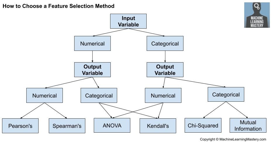
Figure 3. Feature selection strategies
Conclusion
We learned how to inspect the correlation between features using heatmap and select the most informative subset of features using selection methods. The most important takeaway is that irrelevant features must be removed before training a model. If a feature do not contain relevant information or is highly correlated with other features, it will only make the model more complex, less intepretable and you risk reducing the generalization potential of the model.
In the next post we will train our solubility prediction model using the selected features. Can we achieve state-of-the art performance? Stay tuned for the next posts!
Molecular descriptors
https://northstar-www.dartmouth.edu/doc/MOE/Documentation/quasar/descr.htm#KH
http://www.codessa-pro.com/descriptors/index.htm
Feature selection methods
https://machinelearningmastery.com/feature-selection-with-real-and-categorical-data/
Kuhn, Max., and Kjell Johnson. Applied Predictive Modeling. New York: Springer, 2013.
https://www.kaggle.com/willkoehrsen/introduction-to-feature-selection
https://scikit-learn.org/stable/modules/feature_selection.html