Predicting water solubility - Part I?
Primer on Exploratory data analysis.


- Requirements
- Import modules
- Load Data
- Exploratory data analysis
- Detecting outliers
- References
- Fin
- Sample class to sanitize the dataset
Water solubility is one onf the main players in lead optimization. If a molecule is not soluble, we might have problems in biological assays and also to make it reach the desired target in vivo.
This post is the first of a series that will end with a prediction model to estimate water solubility. In this first notebook, we will see some exploratory data analysis and how to prepare a dataset for modeling.
- rdkit >= 2020.09.1
- pandas >= 1.1.3
- seaborn
- matplotlib
- fastcore (!conda install fastcore)
In this tutorial we'll use a dataset compiled by Sorkun et al (2019) from multiple projects to predict water solubility. You can download the original dataset from here.
At the end of the notebook I added a class to process the original dataset in order to remove salts, mixtures, neutralize charges and generate canonical SMILES. I highly recommend checking each structure before modeling.
%reload_ext autoreload
%autoreload 2
%matplotlib inline
from IPython.display import Image
import matplotlib.pyplot as plt
from matplotlib.ticker import FormatStrFormatter
import seaborn as sns
import pandas as pd
import numpy as np
from sklearn.preprocessing import Normalizer, normalize, RobustScaler
from functools import partial
from pathlib import Path
from joblib import load, dump
from scipy import stats
from scipy.stats import norm
from statsmodels.graphics.gofplots import qqplot
from rdkit.Chem import Draw
from rdkit.Chem import MolFromSmiles, MolToSmiles
np.random.seed(5)
sns.set(rc={'figure.figsize': (16, 16)})
sns.set_style('whitegrid')
sns.set_context('paper',font_scale=1.5)
data = pd.read_csv('../_data/curated-solubility-dataset_processed.csv')
data.head()
In this notebook we'll cover three main topics:
- What's the relationship between our features and solubility?
- What's the distribution of our target variable?
- Are there outliers and how can we detect them?
Let's start by counting how many features we have. In total we have 17 descriptors already calculated for our data set.
descriptors = ['MolWt', 'MolLogP', 'MolMR', 'HeavyAtomCount',
'NumHAcceptors', 'NumHDonors', 'NumHeteroatoms', 'NumRotatableBonds',
'NumValenceElectrons', 'NumAromaticRings', 'NumSaturatedRings',
'NumAliphaticRings', 'RingCount', 'TPSA', 'LabuteASA', 'BalabanJ',
'BertzCT']
print(len(descriptors))
We can check the correlation between each feature and solubility using seaborn's regplot:
nr_rows = 6
nr_cols = 3
target = 'Solubility'
fig, axs = plt.subplots(nr_rows, nr_cols, figsize=(nr_cols*3.5,nr_rows*3))
for r in range(0,nr_rows):
for c in range(0,nr_cols):
i = r*nr_cols+c
if i < len(descriptors):
sns.regplot(x=data[descriptors[i]], y=data[target], ax = axs[r][c])
stp = stats.pearsonr(data[descriptors[i]], data[target])
str_title = "r = " + "{0:.2f}".format(stp[0]) + " " "p = " + "{0:.2f}".format(stp[1])
axs[r][c].set_title(str_title,fontsize=11)
plt.tight_layout()
plt.show()

Most have a negative correlation with solubility. In fact, the available features reflect more or less the size/complexity of the molecule (e.g. MolWt, RingCount, MolMR) and it's capacity to make inter and intramolecular interactions (e.g., NumValenceElectrons, NumHAcceptors, NumHDonors, MolLogP), which are known to influence water solubility. For instance, bigger molecules tend to be less soluble in water; the same applies for very liphophilic (aka aversion to water) molecules. On the other hand, more polar molecules, capable of making hydrogen bonds with water molecules, are usually more soluble.
Based on this preliminary analysis we can start thinking which features to include when training a regression model.
Reliability of data
Sorkun et al. described in their paper that the molecules in the dataset were classified according to the number of occurence and the standard deviation of logS measurements. Based on this, the authors considered 5 groups: G1-5, with G5 showing the highest reliability (+3 occurences and SD < 0.5), followed by G4 (+3 occurences and SD > 0.5), G3 (occurences = 2 and SD < 0.5) and G2 (occurences = 2 and SD > 0.5), and finally G1 (just one occurance in all datasets).
Compounds can be classified according to solubility values (LogS); Compounds with 0 and higher solubility value are highly soluble, those in the range of 0 to −2 are soluble, those in the range of −2 to −4 are slightly soluble and insoluble if less than −4.
data['class'] = None
data.loc[data['Solubility']>0.0, 'class'] = 'highly soluble'
data.loc[(data['Solubility']>-2) & (data['Solubility']<=0), 'class'] = 'soluble'
data.loc[(data['Solubility']>-4.0) & (data['Solubility']<=-2.0), 'class'] = 'slightly soluble'
data.loc[data['Solubility']<=-4.0, 'class'] = 'insoluble'
Let's count the molecules in each reliability group.
counts = data.groupby(['Group','class'])['ID'].count().reset_index()
counts
sns.barplot(x='Group',y='ID',data=counts,hue='class',ci=95)

The G1 group dominates, with the majority of molecules, followed by G3 and G5. G4 and G2 are the smallest groups, and contains mostly soluble or slightly soluble molecules. The number of insoluble molecules in all groups is high and comparable to the number of soluble and slighly soluble. In addition, for all groups the number of highly soluble molecules is small; in G2 these molecules represent only 5%.
This initial analysis already shows us that our distribution probably is skewed towards less soluble molecules. This might be a problem when training our model because it might make more errors in the chemical space of highly soluble molecules, since they are not well represented in the dataset.
data.describe()
Let's take a look at the pairplot to see how the features interact with each other and with our target.
sns.pairplot(data)

We can see some interesting information about this dataset. Our target have a normal-like distribution (first plot on the top left). This is very good because some algorithms assume that the data follows a normal distribution. If our data is normal it should be easier to train the model.
Here's another view of the target solubility variable using violin and kernel density plots. The plots shows a negative skew (the distribution shifted to the right), indicating that most molecules are not highly soluble.
fig, (ax1, ax2) = plt.subplots(2,figsize=(12,8))
sns.set_context(font_scale=2)
sns.histplot(x='Solubility',data=data,ax=ax1,hue='class')
ax1.axvline(data['Solubility'].mean(), color='k', linestyle='dashed', linewidth=2.5)
sns.violinplot(data['Solubility'].values,ax=ax2)
# set the spacing between subplots
plt.subplots_adjust(left=0.1,
bottom=0.1,
right=0.9,
top=0.9,
wspace=0.4,
hspace=0.4)
ax1.title.set_text('Histogram')
ax2.title.set_text('Violin plot')
plt.ylabel('Count',fontsize=18)
plt.xlabel('Solubility',fontsize=18)

In order to gain a better insight into our distribution, let's calculate how big is that negative skew and how much the distribution deviates from a Gaussian (normal) distribution. We'll use two values: skewness and kurtosis
Skewness and kurtosis can be defined as follows:
- Skew is how much a distribution is pushed left or right, a measure of asymmetry in the distribution. We can think about skew as if someone was pushing the tail of a normal distribution.
- Kurtosis quantifies how much of the distribution is in the tail. It is a simple and commonly used statistical test for normality. A good analogy is to think about punching the peak or top of the distribution and making it spread to the tails.
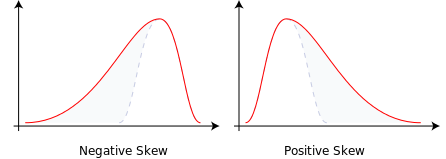
Figure 1. Skewness
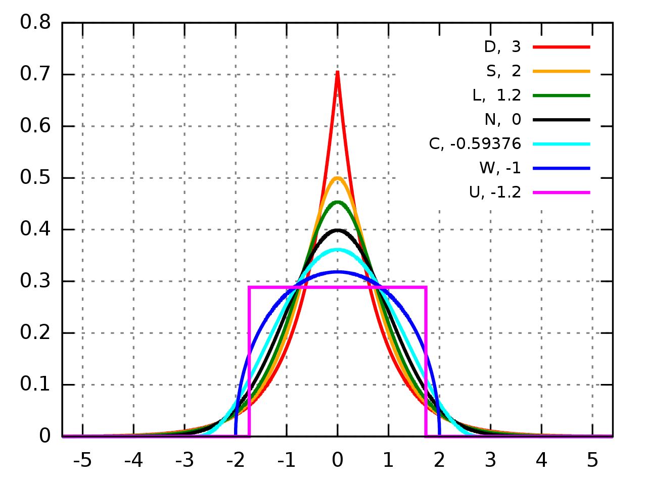
Figure 2. Kurtosis
from scipy.stats import skew, kurtosis, kurtosistest, skewtest
skew_val = skew(data['Solubility'])
kurtosis_val = kurtosis(data['Solubility'])
print(f'Skewness = {skew_val}')
print(f'Kurtosis = {kurtosis_val}')
Now let's confirm the hypothesis that our distribution is not normal. by running different normality tests, such as D'Agostino-Pearson , Shapiro-Wilk and Anderson tests.
from scipy.stats import normaltest, shapiro, anderson
The D'Agostino-Pearson normality test measures how far a distribution is from normality by computing skew and kurtosis. In this test, the null hypothesis (H0) is that our distribution is normal. We can use the k2 statistic and the p-value to reject or not H0.
print("D'Agostino K2")
k2, p = normaltest(data['Solubility'])
print(f'Statistics={k2}, p={p}')
# interpret
alpha = 0.05
if p > alpha:
print('Sample looks Gaussian (fail to reject H0)')
else:
print('Sample does not look Gaussian (reject H0)')
The Shapiro-Wilk normality test calculates a W statistics to check if a sample comes from a normal distribution. In this test, the null hypothesis (H0) is that our distribution is normal. We can use the W statistic and the p-value to reject or not H0.
print("Shapiro-Wilk")
w_stat, p = shapiro(data['Solubility'])
print(f'Statistics={w_stat}, p={p}')
# interpret
alpha = 0.05
if p > alpha:
print('Sample looks Gaussian (fail to reject H0)')
else:
print('Sample does not look Gaussian (reject H0)')
The Anderson-Darling normality test measures if a sample comes from a specific distribution (e.g. normal). It measures the distance between the cumulative probability distribution between the sample and a specific distribution. The test is a modified version of the nonparametric goodness-of-fit Kolmogorov-Smirnov test. In this test, the null hypothesis (H0) is that our distribution is normal. We can use the A statistic and the p-value to reject or not H0. In reality, the scipy function returns a range of critical values that allows us to interpret if H0 should be rejected.
print("Anderson-Darling")
result = anderson(data['Solubility'])
print(f'A statistic = {result.statistic}')
p = 0
for i in range(len(result.critical_values)):
sl, cv = result.significance_level[i], result.critical_values[i]
if result.statistic < result.critical_values[i]:
print(f'{sl:.3f}: {cv:.3f}, data looks normal (fail to reject H0)')
else:
print(f'{sl:.3f}: {cv:.3f}, data does not look normal (reject H0)')
We can also plot some features to investigate their distribution.
fig, ((ax1,ax2),(ax3,ax4)) = plt.subplots(2,2,figsize=(12,12))
sns.histplot(data['MolWt'],ax=ax1)
sns.histplot(data['MolLogP'],ax=ax2)
sns.histplot(data['TPSA'],ax=ax3)
sns.histplot(data['BertzCT'],ax=ax4)
# set the spacing between subplots
plt.subplots_adjust(left=0.1,
bottom=0.1,
right=0.9,
top=0.9,
wspace=0.4,
hspace=0.4)
ax1.set_title('Molecular weight (Da)')
ax2.set_title('Lipophilicity (logP)')
ax3.set_title('Total polar surface area (TPSA)')
ax4.set_title('BertzCT descriptor')

Molecular weight (MolWt), Lipophilicity (MolLogP), total polar surface area (TPSA) and the BertzCT topological descriptor show a clear positive skew. These distributions actually make sense based on our observations about solubility. Most of the molecules in the dataset are in the slightly soluble - soluble range (Solubility between -4 to 0), and as we can see from the above plots, there is a positive skew on molecular weight and lipophilicity.
We can use the information we have to identify data points that are very different from the general distribution and that could hinder the performance of a predictive model. These data points are called outliers and their presence is very bad for many type of algorithms, leading to longer training time, more complex models and maybe degraded performance.
fig, axs = plt.subplots(nr_rows, nr_cols, figsize=(nr_cols*3.5,nr_rows*3))
for r in range(0,nr_rows):
for c in range(0,nr_cols):
i = r*nr_cols+c
if i < len(descriptors):
sns.scatterplot(x=data[descriptors[i]], y=data[target], ax = axs[r][c])
axs[r][c].set_title(descriptors[i],fontsize=11)
plt.tight_layout()
plt.show()

The scatter plots shows us that some points are distant from the others. An extreme case is a data point on the top right of the plots, showing high molecular weight, TPSA and logP! It does seem we have some outliers in our data. But how can we detect which molecules are outliers? Can we simply remove them based on some kind of rule of thumb? Let's investigate this!
c = 2
def get_outliers(data, feature_name, c=2):
mean, std = data[feature_name].mean(),data[feature_name].std()
bounds = mean - (c*std), mean + (c*std)
outliers = data[~data[feature_name].between(*bounds)]
non_outliers = data.iloc[data.index.difference(outliers.index)]
return bounds, outliers, non_outliers
outliers = []
for i in descriptors:
outliers.append(get_outliers(data, feature_name= i, c=2)[1])
fig, axs = plt.subplots(nr_rows, nr_cols, figsize=(nr_cols*3.5,nr_rows*3))
for r in range(0,nr_rows):
for c in range(0,nr_cols):
i = r*nr_cols+c
if i < len(descriptors):
sns.scatterplot(x=data[descriptors[i]], y=data[target], ax = axs[r][c])
sns.scatterplot(x=outliers[i][descriptors[i]], y=outliers[i][target], ax = axs[r][c])
# print(f'Possible number of outliers = {}')
axs[r][c].set_title(f'{descriptors[i]}\nNumber of outliers = {len(outliers[i])}',fontsize=11)
# set the spacing between subplots
plt.subplots_adjust(left=0.1,
bottom=0.1,
right=0.9,
top=0.9,
wspace=0.4,
hspace=0.4)
plt.tight_layout()
plt.show()

The scatterplots shows some potential outliers for each feature.
Let's take a closer look at solubility and one of the descriptor to get some insight of physicochemical properties of potential outliers.
Water solubility has a strong negative correlation with lipophilicity (logP). Ideally, we should see a solubility decrease for more lipophilic molecules. Let's try using logP to identify potential outliers.
logp_bonds,logp_outliers,logp_non_outliers = get_outliers(data, feature_name= 'MolLogP', c=2)
print(logp_bonds)
print(f'Possible number of outliers = {len(logp_outliers)}')
We found 300 potential outliers that differ from the mean MolLogP by 2 std. We can clearly see the extreme point we identified earlier and some other more distant fromt he distribution.
Here's MolLogP before and after outliers
fig, ax1 = plt.subplots(1,figsize=(20,16), sharey=True)
s=90
sns.scatterplot(x='MolLogP', y='Solubility', data =logp_non_outliers,ax=ax1,s=s,color='gray')
sns.scatterplot(x='MolLogP', y='Solubility', data =logp_outliers,ax=ax1,color='goldenrod',s=s)
ax1.set_title('MolLogP outliers',fontsize=18)
ax1.set_ylabel('Solubility',fontsize=18)
ax1.set_xlabel('MolLogP',fontsize=18)
#sns.scattrplot(x='MolLogP', y='Solubility', data = logp_non_outliers,ax=ax3,color='gray')
#ax3.set_title('Removed outliers')

If we remove the putative outliers we can get a better view of the relationship between logP and solubility.
fig, (ax1, ax2, ax3) = plt.subplots(1,3,figsize=(36,12), sharey=True)
s=90
sns.scatterplot(x='MolLogP', y='Solubility', data =data,ax=ax1,s=s,color='gray')
ax1.set_title('Original data')
sns.scatterplot(x='MolLogP', y='Solubility', data =logp_non_outliers,ax=ax2,s=s,color='gray')
sns.scatterplot(x='MolLogP', y='Solubility', data =logp_outliers,ax=ax2,color='goldenrod',s=s)
ax2.set_title('Outliers')
sns.scatterplot(x='MolLogP', y='Solubility', data = logp_non_outliers,ax=ax3,color='gray')
ax3.set_title('Removed outliers')

The scatterplot on the right shows that as logP increases, the solubility tends to decrease, which is what we expected. In general, very big compounds are less soluble and have a hard time being optimized into lead compounds or drugs. But what kind of molecules did we remove?
from rdkit.Chem import Draw
Draw.MolsToGridImage(list(map(MolFromSmiles, logp_outliers.processed_smiles)),subImgSize=(900,900))

Some potential outliers doesn't look very friendly or something that would be in drug discovery libraries! Take a look at this guy:
smi = logp_outliers.processed_smiles.tolist()[2]
mol = MolFromSmiles(smi)
print(f'Outlier SMILES - {smi}')
mol

We might be better off without this kind of "ugly chemistry". But let's keep these monsters for now and explore other methods to outlier detection.
def iqr_detection(data, feature_name, std_cut=1.5):
df = data.copy()
df.reset_index(drop=True,inplace=True)
q3 = np.quantile(df[feature_name],.75)
q1 = np.quantile(df[feature_name],.25)
iqr = q3 - q1
cutoff = std_cut * iqr
lower, upper = q1 - cutoff, q3 + cutoff
outliers = df[(df[feature_name] < lower) | (df[feature_name] > upper)]
ok_points = df.iloc[df.index.difference(outliers.index)]
return (lower, upper), outliers, ok_points
We will consider a data point as outlier if it lies at above or below the cutoff value of 1.5 * IQR
iqr_bounds, iqr_outliers, iqr_okpoints = iqr_detection(data, 'Solubility')
print(iqr_bounds)

Automatic detection
We can also automate the detection of outliers using the local outlier factor algorithm
The local outlier factor (LOF) adopts a notion of oulier that depends on the local neighborhood of each data point. This allows the algorithm to find data points that are different from the global distribution and also different from their neighbors. LOF does this by assigning an outlier factor to each data point, which is the degree each point deviates from its neighbors. An outlier is expected to have a local densitiy that is smaller (its far away) from it's k-neighbors.
Let's try to find some outliers with the available descriptors. But first, let's normalize them!
X = data[descriptors].values
Y = data['Solubility'].values
Y.shape
scaler = RobustScaler()
Xnorm = scaler.fit(X).transform(X)
Xnorm.mean(),Xnorm.std()
from sklearn.neighbors import LocalOutlierFactor
outlier_scores = LocalOutlierFactor(n_neighbors=20,novelty=False).fit_predict(Xnorm)
lof_no_outliers = data.iloc[outlier_scores == 1]
lof_outliers = data.iloc[outlier_scores == -1]
lof_no_outliers.shape,lof_outliers.shape
Draw.MolsToGridImage(list(map(MolFromSmiles, lof_outliers.processed_smiles.tolist())),subImgSize=(600,600))


It seems LOF removed the most extreme points. After removing outliers, we can see that the correlation between each feature and solubility increased. The only exception was TPSA, which showed a small decrease in the Pearson's correlation.
In the next posts, we'll explore more of this data. The main question we'll try to answer is: can we train a model with good performance to predict water solubility?
Detecting outliers
https://www.ucd.ie/ecomodel/Resources/QQplots_WebVersion.html
https://www.dummies.com/programming/big-data/data-science/graphical-tests-of-data-outliers/
https://machinelearningmastery.com/how-to-use-statistics-to-identify-outliers-in-data/
https://towardsdatascience.com/ways-to-detect-and-remove-the-outliers-404d16608dba
https://www.dbs.ifi.lmu.de/Publikationen/Papers/LOF.pdf
https://towardsdatascience.com/local-outlier-factor-for-anomaly-detection-cc0c770d2ebe
Normality tests
Machine learning mastery post: https://machinelearningmastery.com/a-gentle-introduction-to-normality-tests-in-python/
Shapiro-Wilk test: https://www.itl.nist.gov/div898/handbook/prc/section2/prc213.htm
Anderson-Darling test : https://www.itl.nist.gov/div898/handbook/prc/section2/prc21.htm
GraphPad entry: https://www.graphpad.com/guides/prism/latest/statistics/stat_choosing_a_normality_test.htm
from unittest.mock import *
from rdkit import Chem
from tqdm.notebook import tqdm
from rdkit.Chem.Draw import IPythonConsole, MolsToGridImage
from rdkit.Chem.SaltRemover import SaltRemover as saltremover
from rdkit.Chem.MolStandardize.rdMolStandardize import LargestFragmentChooser
from rdkit.Chem import AllChem, SanitizeMol
from rdkit import rdBase
from rdkit.Chem import rdmolops
from fastcore.all import *
rdBase.DisableLog('rdApp.error')
rdBase.DisableLog('rdApp.info')
_saltremover = saltremover()
_unwanted = Chem.MolFromSmarts('[!#1!#6!#7!#8!#9!#15!#16!#17!#35!#53]')
def _initialiseNeutralisationReactions():
patts = (
# Imidazoles
('[n+;H]', 'n'),
# Amines
('[N+;!H0]', 'N'),
# Carboxylic acids and alcohols
('[$([O-]);!$([O-][#7])]', 'O'),
# Thiols
('[S-;X1]', 'S'),
#Amidines
('[C+](N)', 'C(=N)'),
# Sulfonamides
('[$([N-;X2]S(=O)=O)]', 'N'),
# Enamines
('[$([N-;X2][C,N]=C)]', 'N'),
# Tetrazoles
('[n-]', '[nH]'),
# Sulfoxides
('[$([S-]=O)]', 'S'),
# Amides
('[$([N-]C=O)]', 'N'),
)
return [(Chem.MolFromSmarts(x),Chem.MolFromSmiles(y,False)) for x,y in patts]
def neutralise(mol,reactions=None):
reactions = _initialiseNeutralisationReactions()
replaced = False
for i,(reactant, product) in enumerate(reactions):
while mol.HasSubstructMatch(reactant):
replaced = True
rms = AllChem.ReplaceSubstructs(mol, reactant, product)
mol = rms[0]
if replaced:
rdmolops.Cleanup(mol)
rdmolops.SanitizeMol(mol)
mol = rdmolops.RemoveHs(mol, implicitOnly=False, updateExplicitCount=False, sanitize=True)
return mol
else:
rdmolops.Cleanup(mol)
rdmolops.SanitizeMol(mol)
mol = rdmolops.RemoveHs(mol, implicitOnly=False, updateExplicitCount=False, sanitize=True)
return mol
def _rare_filters(mol):
if mol:
cyano_filter = "[C-]#[N+]"
oh_filter = "[OH+]"
sulfur_filter = "[SH]"
sulfur_filter2 = "[SH2]"
iodine_filter1 = "[IH2]"
iodine_filter2 = "[I-]"
iodine_filter3 = "[I+]"
if not mol.HasSubstructMatch(Chem.MolFromSmarts(cyano_filter)) \
and not mol.HasSubstructMatch(Chem.MolFromSmarts(oh_filter)) \
and not mol.HasSubstructMatch(Chem.MolFromSmarts(sulfur_filter2)) \
and not mol.HasSubstructMatch(Chem.MolFromSmarts(iodine_filter1)) \
and not mol.HasSubstructMatch(Chem.MolFromSmarts(iodine_filter2)) \
and not mol.HasSubstructMatch(Chem.MolFromSmarts(iodine_filter3)) \
and not mol.HasSubstructMatch(Chem.MolFromSmarts(sulfur_filter)):
return mol
def set_active(row):
active = 'Inactive'
if row['standard_value'] <= 10000: active = 'Active'
return active
class SanitizeDataset():
def __init__(self,df,smiles_column:str='Smiles',activity_column = None, sep:str='\t'):
self.df, self.smiles_column, self.activity_column = df, smiles_column, activity_column
@patch
@delegates(SanitizeDataset)
def add_mol_column(x:SanitizeDataset, smiles, **kwargs):
if type(smiles) == str and smiles != '':
mol = Chem.MolFromSmiles(smiles) #.replace('@','').replace('/','').replace("\\","")
return mol
else:
return None
@patch
@delegates(SanitizeDataset)
def remove_unwanted(x:SanitizeDataset,mol, **kwargs):
if not mol.HasSubstructMatch(_unwanted) and (sum([atom.GetIsotope() for atom in mol.GetAtoms()])==0):
return mol
@patch
@delegates(SanitizeDataset)
def _remove_salts(x:SanitizeDataset,mol, **kwargs):
mol = _saltremover.StripMol(mol, dontRemoveEverything=True)
mol = _saltremover.StripMol(mol, dontRemoveEverything=True)
mol = rdmolops.RemoveHs(mol, implicitOnly=False, updateExplicitCount=False, sanitize=True)
mol = x._getlargestFragment(mol)
return mol
@patch
@delegates(SanitizeDataset)
def _getlargestFragment(x:SanitizeDataset, mol, **kwargs):
frags = rdmolops.GetMolFrags(mol, asMols=True, sanitizeFrags=True)
maxmol = None
for mol in frags:
if mol is None:
continue
if maxmol is None:
maxmol = mol
if maxmol.GetNumHeavyAtoms() < mol.GetNumHeavyAtoms():
maxmol = mol
return maxmol
@patch
@delegates(SanitizeDataset)
def is_valid(x:SanitizeDataset, mol, min_heavy_atoms = 1, max_heavy_atoms = 9999, **kwargs):
if mol:
return _rare_filters(mol) if min_heavy_atoms < mol.GetNumHeavyAtoms() < max_heavy_atoms else None
return None
@patch
@delegates(SanitizeDataset)
def canonilize(x:SanitizeDataset, mol, **kwargs):
if mol:
return Chem.MolToSmiles(mol, isomericSmiles = True) if mol.GetNumHeavyAtoms()>0 else print(type(mol))
else:
return None
@patch
@delegates(SanitizeDataset)
def process_data(x:SanitizeDataset, **kwargs):
x.df = x.df.loc[~x.df[x.smiles_column].isnull()]
x.df['mol'] = x.df[x.smiles_column].apply(x.add_mol_column)
x.df = x.df.loc[~x.df['mol'].isnull()]
x.df['mol'] = x.df['mol'].apply(x.remove_unwanted)
x.df['mol'] = x.df['mol'].apply(_rare_filters)
x.df = x.df.loc[~x.df['mol'].isnull()]
x.df['mol'] = x.df['mol'].apply(x._remove_salts)
x.df['mol'] = x.df['mol'].apply(neutralise)
x.df['mol'] = x.df['mol'].apply(x.is_valid)
x.df = x.df.loc[~x.df['mol'].isnull()]
x.df['processed_smiles'] = x.df['mol'].apply(lambda x : Chem.MolToSmiles(x))
x.df = x.df.loc[~x.df['processed_smiles'].isnull()]
x.df.drop_duplicates(subset='processed_smiles',inplace=True)
return x.df
#sanitizer = SanitizeDataset(df=df, smiles_column='SMILES',activity_column = 'Solubility', sep=',')